# Simulated example data (two groups, simple outcome)
set.seed(42)
n <- 400
simdat <- tibble(
  group = sample(c("Control", "Treatment"), n, TRUE),
  x = rnorm(n),
  y = 0.4 * (group == "Treatment") + 0.6 * x + rnorm(n, sd = 0.8)
)

# A small model for diagnostic plots later
mod <- lm(y ~ x + group, data = simdat)
simdat$.fitted <- fitted(mod)
simdat$.resid  <- resid(mod)

# Penguins subset (complete cases)
peng <- penguins |>
  select(species, island, bill_length_mm, bill_depth_mm, body_mass_g, flipper_length_mm, sex) |>
drop_na()GC3 Roundtable #3 — Layout and Composition of Multiple Plots
From Single Figures to Cohesive Visual Stories
Why layout matters
- Last time: group comparisons (e.g., violin/box/raincloud).
- Today: how multiple plots work together to tell one story.
- Good layout ⇒ stronger visual hierarchy, comparability, and clarity.
- Bad layout ⇒ clutter, duplicated elements, and misinterpretation.
Note
Goal: Compose multi-panel figures that are publication-ready and reproducible.
What we’ll cover
- Patchwork grammar for multi-plot composition
- Advanced control: widths/heights, custom designs, legend & axis collection
- Design principles: hierarchy, accessibility, and story flow
- Demos: diagnostics dashboard, group comparisons, publication figure with tags
- Exporting & common pitfalls
Packages for layout
| Package | Strength | Example |
|---|---|---|
| patchwork | Intuitive grammar & guide/axis collection | (p1 | p2) / p3 |
| cowplot | Precise alignment; plot grids | plot_grid(p1, p2) |
| gridExtra | Base grid layouts | grid.arrange(p1, p2) |
We’ll primarily use patchwork.
Data used in demos
We’ll mix simulated data and palmerpenguins.
Patchwork basics: horizontal & vertical
p1 <- ggplot(simdat, aes(group, y, fill = group)) +
  geom_violin(trim = FALSE, alpha = 0.6) +
  geom_boxplot(width = 0.2, outlier.shape = NA) +
  labs(title = "Outcome by Group") +
  theme(legend.position = "none")

p2 <- ggplot(simdat, aes(x, y, color = group)) +
  geom_point(alpha = 0.5) +
  geom_smooth(method = "lm", se = FALSE) +
  labs(title = "x vs y by Group")
# Side-by-side (horizontal)
p1 | p2`geom_smooth()` using formula = 'y ~ x'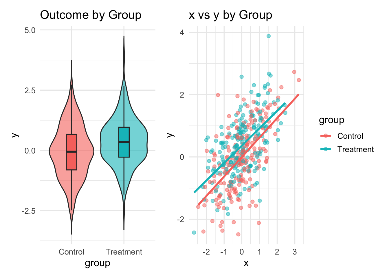
# Stacked (vertical)
p1 / p2
`geom_smooth()` using formula = 'y ~ x'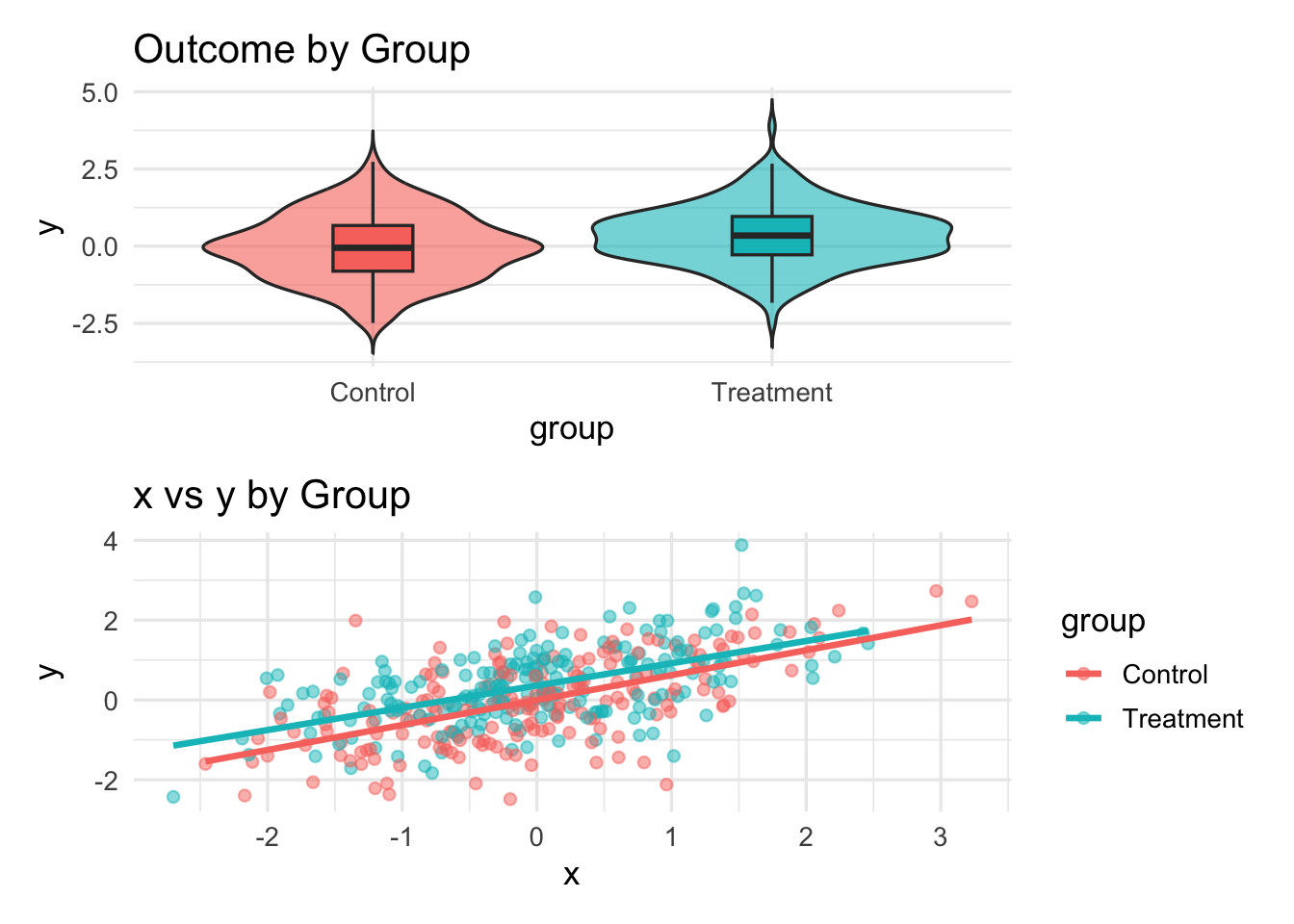
Patchwork: nesting & layout
# Mixed nesting
(p1 | p2) / (p2 | p1)
`geom_smooth()` using formula = 'y ~ x'
`geom_smooth()` using formula = 'y ~ x'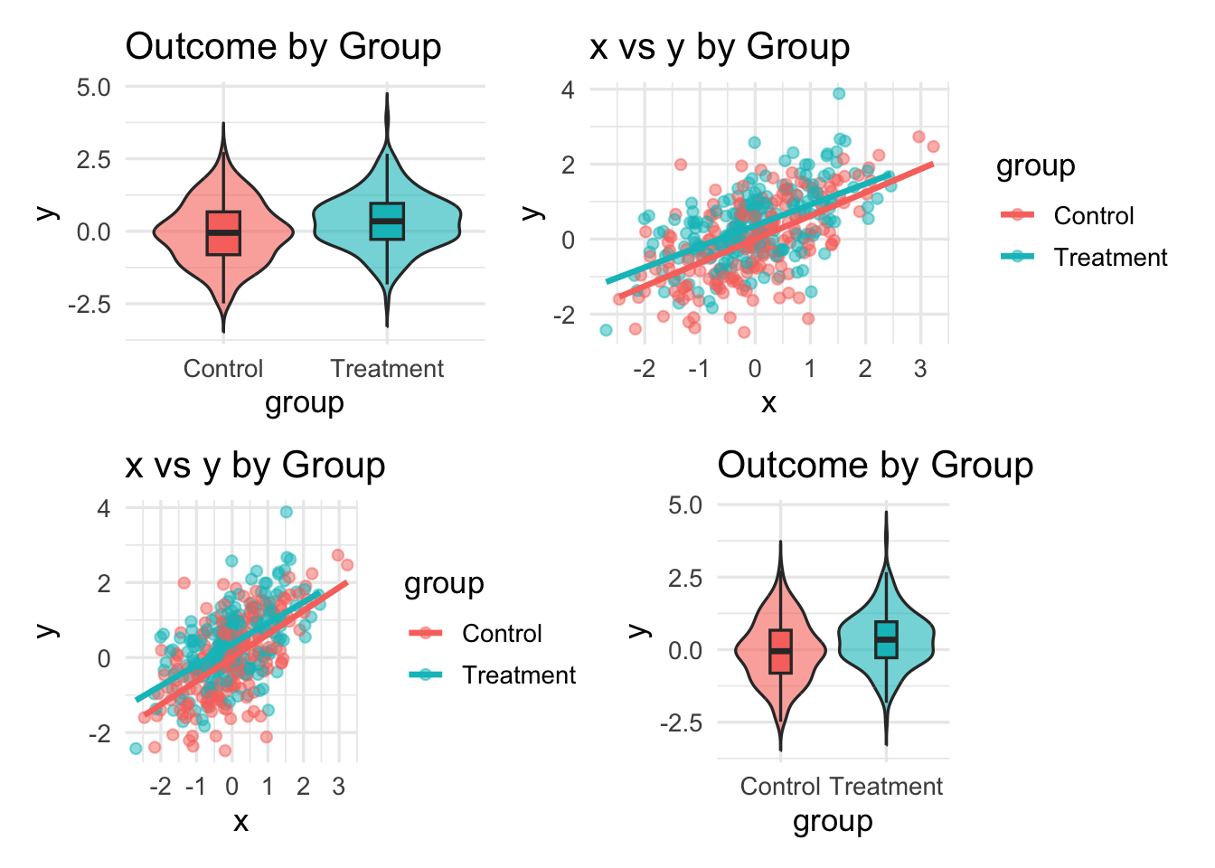
# Specify grid dimensions
(p1 | p2 | p1) + plot_layout(ncol = 3)
`geom_smooth()` using formula = 'y ~ x'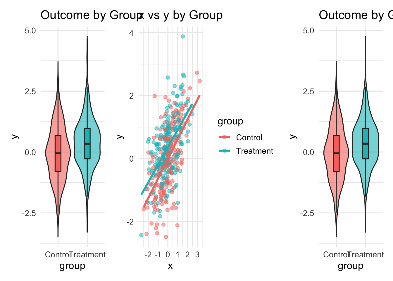
# Control relative widths / heights
(p1 | p2) + plot_layout(widths = c(1.2, 1))
`geom_smooth()` using formula = 'y ~ x'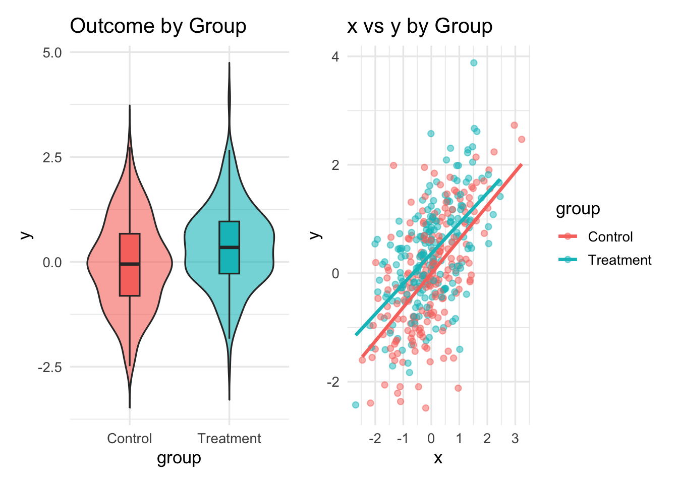
Custom designs & spacers
# Custom layout design string
design <- "
AAB
CCD
"

p3 <- ggplot(simdat, aes(x = .fitted, y = .resid, color = group)) +
  geom_point(alpha = 0.6) +
  geom_hline(yintercept = 0, linetype = 2) +
  labs(title = "Residuals vs Fitted")

p4 <- ggplot(simdat, aes(sample = .resid, color = group)) +
  stat_qq(alpha = 0.6) +
  stat_qq_line() +
  labs(title = "Q-Q Plot (Residuals)")

p1 + p2 + p3 + p4 + plot_layout(design = design)
`geom_smooth()` using formula = 'y ~ x'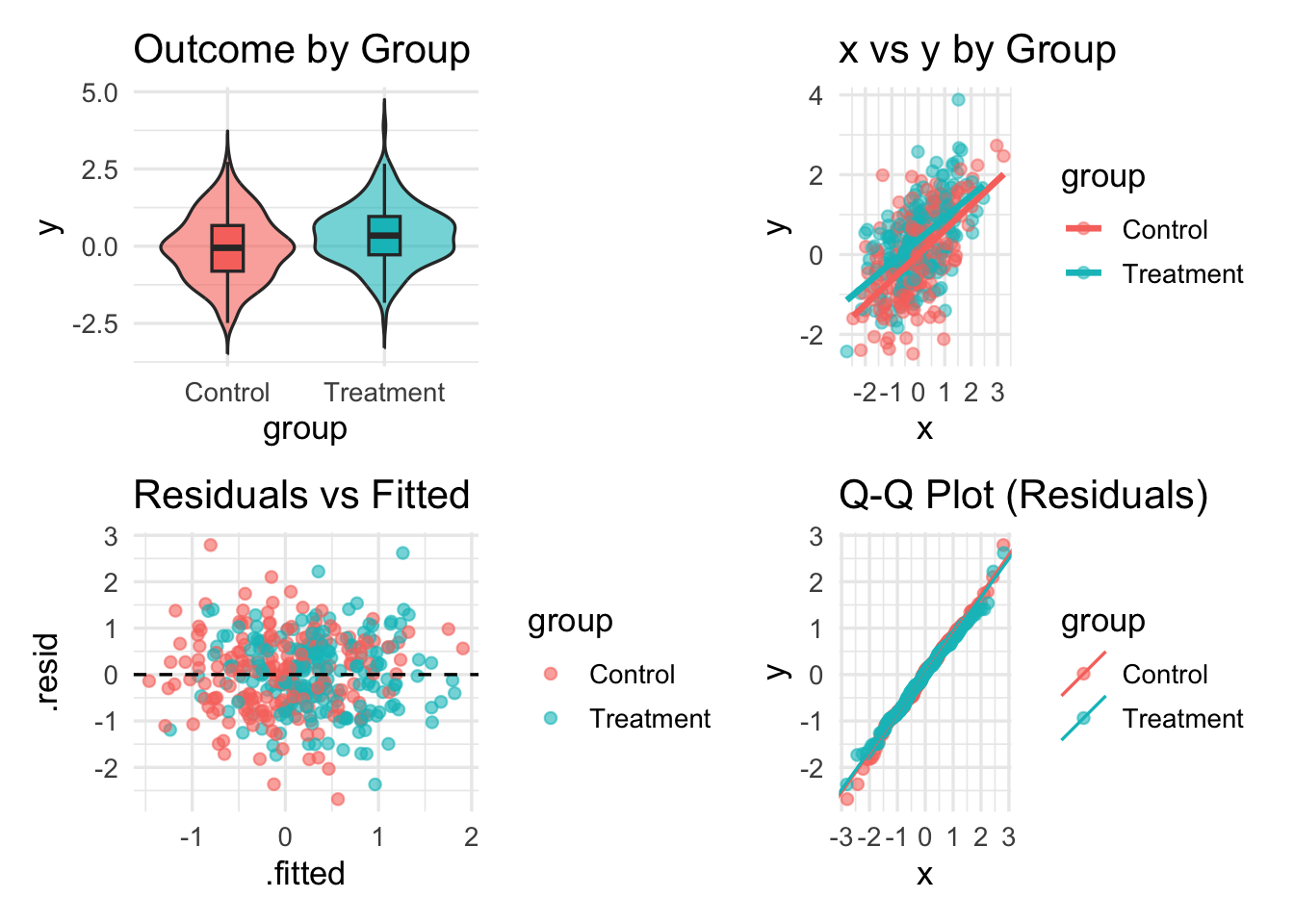
# Spacers for intentional whitespace
p1 | plot_spacer() | p2
`geom_smooth()` using formula = 'y ~ x'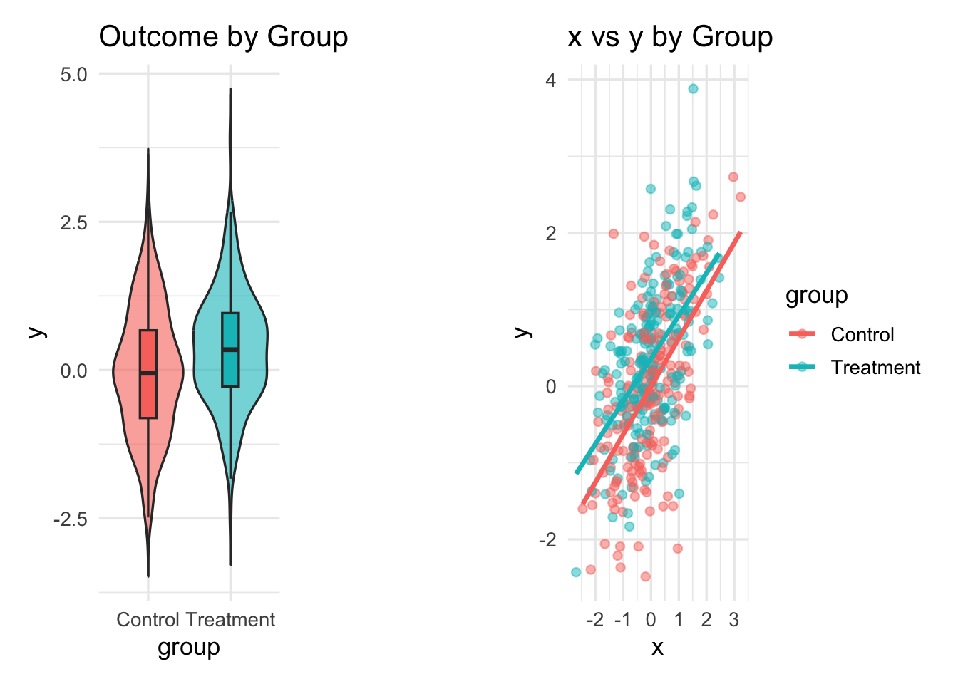
Collecting legends & axes
# Legends: collect across panels
(p2 | p3 | p4) +
  plot_layout(guides = "collect") +
  plot_annotation(title = "Diagnostics with Shared Legend")
`geom_smooth()` using formula = 'y ~ x'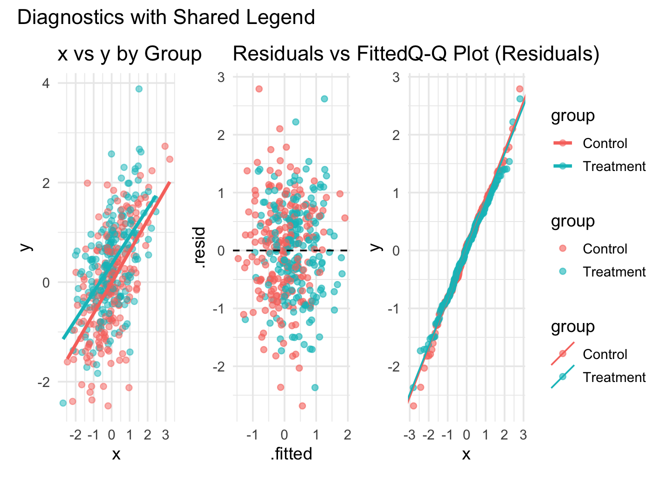
# Global theme tweaks via '&'
((p2 | p3) / p4) &
  theme(legend.position = "bottom",
        plot.title.position = "plot")
`geom_smooth()` using formula = 'y ~ x'
Demo: Diagnostics dashboard
diag1 <- ggplot(simdat, aes(.fitted, .resid, color = group)) +
  geom_point(alpha = 0.6) +
  geom_hline(yintercept = 0, linetype = 2) +
  labs(x = "Fitted", y = "Residuals", title = "Residuals vs Fitted")

diag2 <- ggplot(simdat, aes(x = .resid, fill = group)) +
  geom_histogram(position = "identity", alpha = 0.5, bins = 30) +
  labs(x = "Residual", title = "Residual Distribution")

diag3 <- ggplot(simdat, aes(sample = .resid, color = group)) +
  stat_qq(alpha = 0.5) + stat_qq_line() +
  labs(title = "Q–Q Plot")

(diag1 | diag2 | diag3) +
  plot_layout(guides = "collect") +
  plot_annotation(title = "Model Diagnostics Overview")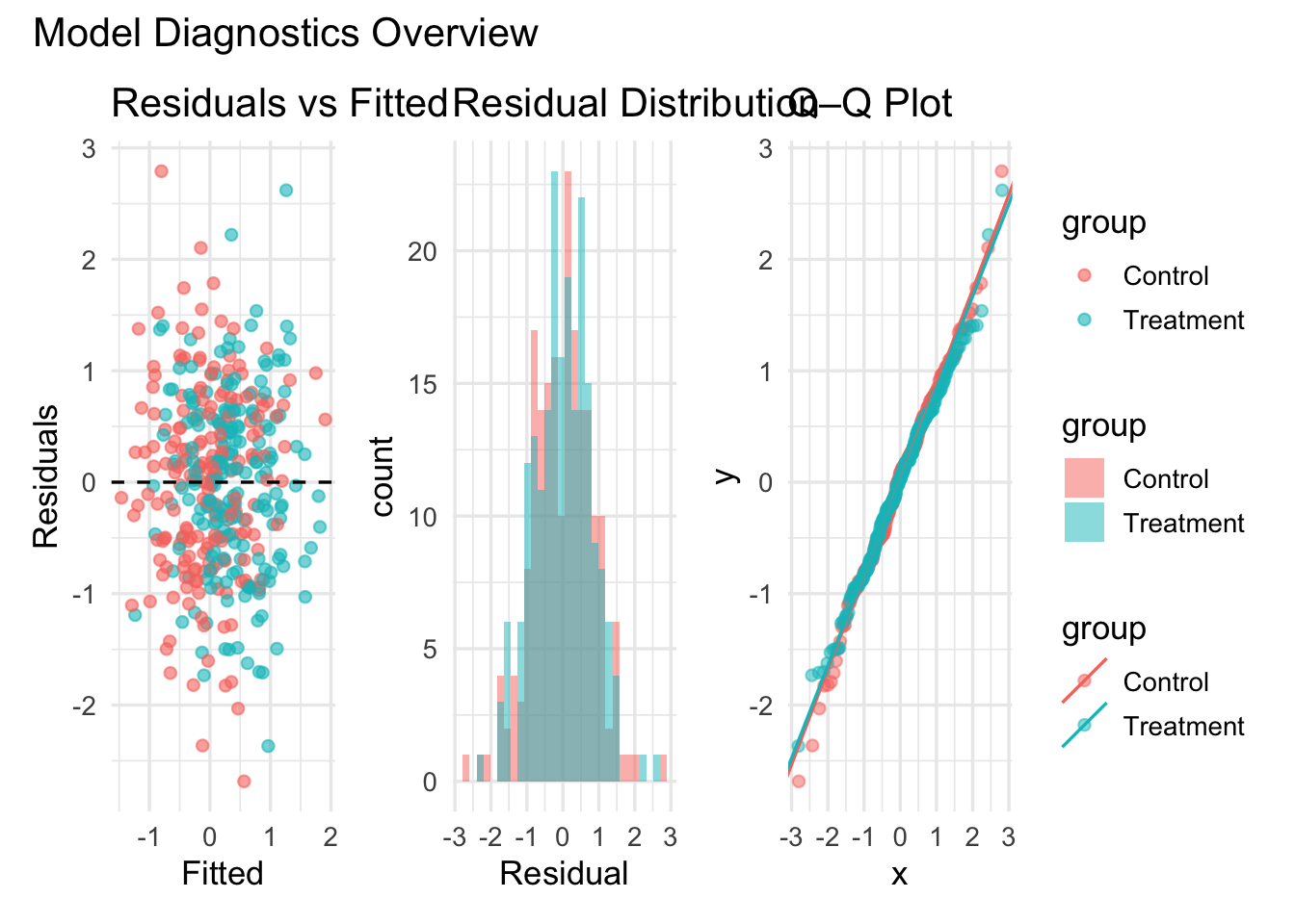
Demo: Group comparisons panel (penguins)
gA <- ggplot(peng, aes(species, bill_length_mm, fill = species)) +
  geom_violin(trim = FALSE, alpha = 0.6) +
  geom_boxplot(width = 0.15, outlier.shape = NA) +
  labs(title = "Bill Length by Species", x = NULL, y = "mm")

gB <- ggplot(peng, aes(species, bill_depth_mm, fill = species)) +
  geom_violin(trim = FALSE, alpha = 0.6) +
  geom_boxplot(width = 0.15, outlier.shape = NA) +
  labs(title = "Bill Depth by Species", x = NULL, y = "mm")

gC <- ggplot(peng, aes(species, body_mass_g, fill = species)) +
  geom_violin(trim = FALSE, alpha = 0.6) +
  geom_boxplot(width = 0.15, outlier.shape = NA) +
  labs(title = "Body Mass by Species", x = NULL, y = "g")

(gA | gB | gC) +
  plot_layout(guides = "collect") +
  plot_annotation(title = "Morphological Differences Among Penguin Species")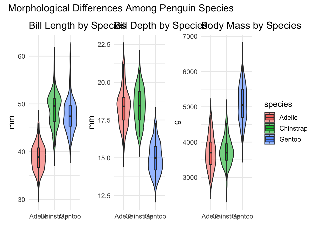
Publication-ready figure: tags & hierarchy
pub <- ((gA | gB) / (gC | diag1)) +
  plot_layout(guides = "collect", heights = c(1, 1.1)) +
  plot_annotation(title = "Figure 2. Study Results Summary",
                  tag_levels = "A")

pub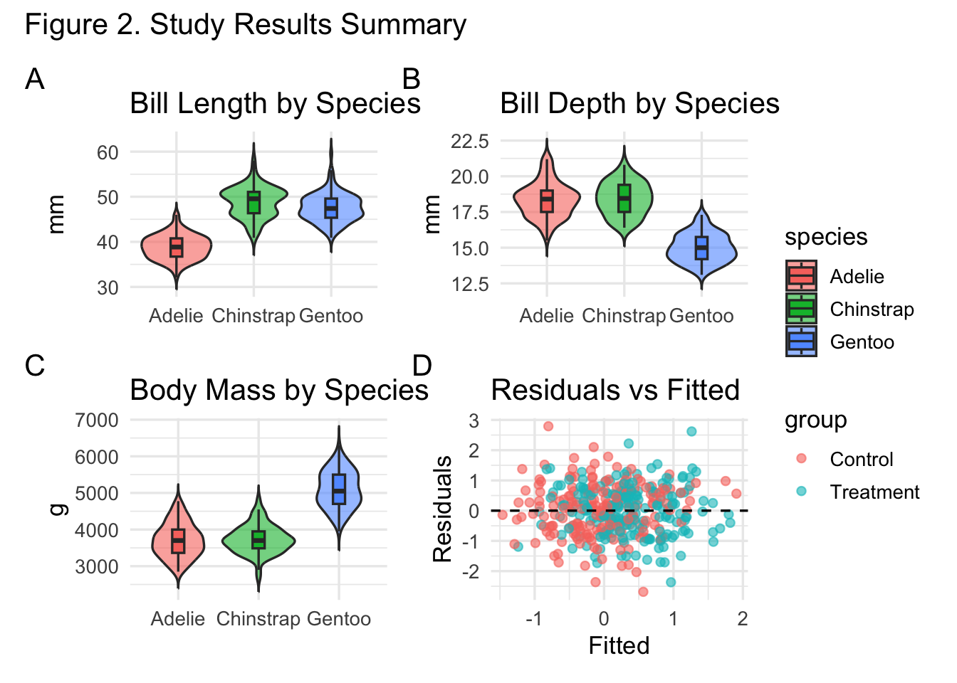
Mixing plots with a table
tbl <- peng |>
  group_by(species) |>
  summarize(n = n(),
            mean_mass = round(mean(body_mass_g), 1),
            mean_bill = round(mean(bill_length_mm), 1),
            .groups = "drop") |>
  arrange(desc(n)) |>
  gt() |>
  tab_header(title = "Sample Summary by Species")

# Render table to graphic (cowplot) for composition
tbl_grob <- cowplot::ggdraw() + cowplot::draw_grob(grid::grid.grabExpr(print(tbl)))
<div id="obmldgmsmz" style="padding-left:0px;padding-right:0px;padding-top:10px;padding-bottom:10px;overflow-x:auto;overflow-y:auto;width:auto;height:auto;">
<style>#obmldgmsmz table {
font-family: system-ui, 'Segoe UI', Roboto, Helvetica, Arial, sans-serif, 'Apple Color Emoji', 'Segoe UI Emoji', 'Segoe UI Symbol', 'Noto Color Emoji';
-webkit-font-smoothing: antialiased;
-moz-osx-font-smoothing: grayscale;
}
#obmldgmsmz thead, #obmldgmsmz tbody, #obmldgmsmz tfoot, #obmldgmsmz tr, #obmldgmsmz td, #obmldgmsmz th {
border-style: none;
}
#obmldgmsmz p {
margin: 0;
padding: 0;
}
#obmldgmsmz .gt_table {
display: table;
border-collapse: collapse;
line-height: normal;
margin-left: auto;
margin-right: auto;
color: #333333;
font-size: 16px;
font-weight: normal;
font-style: normal;
background-color: #FFFFFF;
width: auto;
border-top-style: solid;
border-top-width: 2px;
border-top-color: #A8A8A8;
border-right-style: none;
border-right-width: 2px;
border-right-color: #D3D3D3;
border-bottom-style: solid;
border-bottom-width: 2px;
border-bottom-color: #A8A8A8;
border-left-style: none;
border-left-width: 2px;
border-left-color: #D3D3D3;
}
#obmldgmsmz .gt_caption {
padding-top: 4px;
padding-bottom: 4px;
}
#obmldgmsmz .gt_title {
color: #333333;
font-size: 125%;
font-weight: initial;
padding-top: 4px;
padding-bottom: 4px;
padding-left: 5px;
padding-right: 5px;
border-bottom-color: #FFFFFF;
border-bottom-width: 0;
}
#obmldgmsmz .gt_subtitle {
color: #333333;
font-size: 85%;
font-weight: initial;
padding-top: 3px;
padding-bottom: 5px;
padding-left: 5px;
padding-right: 5px;
border-top-color: #FFFFFF;
border-top-width: 0;
}
#obmldgmsmz .gt_heading {
background-color: #FFFFFF;
text-align: center;
border-bottom-color: #FFFFFF;
border-left-style: none;
border-left-width: 1px;
border-left-color: #D3D3D3;
border-right-style: none;
border-right-width: 1px;
border-right-color: #D3D3D3;
}
#obmldgmsmz .gt_bottom_border {
border-bottom-style: solid;
border-bottom-width: 2px;
border-bottom-color: #D3D3D3;
}
#obmldgmsmz .gt_col_headings {
border-top-style: solid;
border-top-width: 2px;
border-top-color: #D3D3D3;
border-bottom-style: solid;
border-bottom-width: 2px;
border-bottom-color: #D3D3D3;
border-left-style: none;
border-left-width: 1px;
border-left-color: #D3D3D3;
border-right-style: none;
border-right-width: 1px;
border-right-color: #D3D3D3;
}
#obmldgmsmz .gt_col_heading {
color: #333333;
background-color: #FFFFFF;
font-size: 100%;
font-weight: normal;
text-transform: inherit;
border-left-style: none;
border-left-width: 1px;
border-left-color: #D3D3D3;
border-right-style: none;
border-right-width: 1px;
border-right-color: #D3D3D3;
vertical-align: bottom;
padding-top: 5px;
padding-bottom: 6px;
padding-left: 5px;
padding-right: 5px;
overflow-x: hidden;
}
#obmldgmsmz .gt_column_spanner_outer {
color: #333333;
background-color: #FFFFFF;
font-size: 100%;
font-weight: normal;
text-transform: inherit;
padding-top: 0;
padding-bottom: 0;
padding-left: 4px;
padding-right: 4px;
}
#obmldgmsmz .gt_column_spanner_outer:first-child {
padding-left: 0;
}
#obmldgmsmz .gt_column_spanner_outer:last-child {
padding-right: 0;
}
#obmldgmsmz .gt_column_spanner {
border-bottom-style: solid;
border-bottom-width: 2px;
border-bottom-color: #D3D3D3;
vertical-align: bottom;
padding-top: 5px;
padding-bottom: 5px;
overflow-x: hidden;
display: inline-block;
width: 100%;
}
#obmldgmsmz .gt_spanner_row {
border-bottom-style: hidden;
}
#obmldgmsmz .gt_group_heading {
padding-top: 8px;
padding-bottom: 8px;
padding-left: 5px;
padding-right: 5px;
color: #333333;
background-color: #FFFFFF;
font-size: 100%;
font-weight: initial;
text-transform: inherit;
border-top-style: solid;
border-top-width: 2px;
border-top-color: #D3D3D3;
border-bottom-style: solid;
border-bottom-width: 2px;
border-bottom-color: #D3D3D3;
border-left-style: none;
border-left-width: 1px;
border-left-color: #D3D3D3;
border-right-style: none;
border-right-width: 1px;
border-right-color: #D3D3D3;
vertical-align: middle;
text-align: left;
}
#obmldgmsmz .gt_empty_group_heading {
padding: 0.5px;
color: #333333;
background-color: #FFFFFF;
font-size: 100%;
font-weight: initial;
border-top-style: solid;
border-top-width: 2px;
border-top-color: #D3D3D3;
border-bottom-style: solid;
border-bottom-width: 2px;
border-bottom-color: #D3D3D3;
vertical-align: middle;
}
#obmldgmsmz .gt_from_md > :first-child {
margin-top: 0;
}
#obmldgmsmz .gt_from_md > :last-child {
margin-bottom: 0;
}
#obmldgmsmz .gt_row {
padding-top: 8px;
padding-bottom: 8px;
padding-left: 5px;
padding-right: 5px;
margin: 10px;
border-top-style: solid;
border-top-width: 1px;
border-top-color: #D3D3D3;
border-left-style: none;
border-left-width: 1px;
border-left-color: #D3D3D3;
border-right-style: none;
border-right-width: 1px;
border-right-color: #D3D3D3;
vertical-align: middle;
overflow-x: hidden;
}
#obmldgmsmz .gt_stub {
color: #333333;
background-color: #FFFFFF;
font-size: 100%;
font-weight: initial;
text-transform: inherit;
border-right-style: solid;
border-right-width: 2px;
border-right-color: #D3D3D3;
padding-left: 5px;
padding-right: 5px;
}
#obmldgmsmz .gt_stub_row_group {
color: #333333;
background-color: #FFFFFF;
font-size: 100%;
font-weight: initial;
text-transform: inherit;
border-right-style: solid;
border-right-width: 2px;
border-right-color: #D3D3D3;
padding-left: 5px;
padding-right: 5px;
vertical-align: top;
}
#obmldgmsmz .gt_row_group_first td {
border-top-width: 2px;
}
#obmldgmsmz .gt_row_group_first th {
border-top-width: 2px;
}
#obmldgmsmz .gt_summary_row {
color: #333333;
background-color: #FFFFFF;
text-transform: inherit;
padding-top: 8px;
padding-bottom: 8px;
padding-left: 5px;
padding-right: 5px;
}
#obmldgmsmz .gt_first_summary_row {
border-top-style: solid;
border-top-color: #D3D3D3;
}
#obmldgmsmz .gt_first_summary_row.thick {
border-top-width: 2px;
}
#obmldgmsmz .gt_last_summary_row {
padding-top: 8px;
padding-bottom: 8px;
padding-left: 5px;
padding-right: 5px;
border-bottom-style: solid;
border-bottom-width: 2px;
border-bottom-color: #D3D3D3;
}
#obmldgmsmz .gt_grand_summary_row {
color: #333333;
background-color: #FFFFFF;
text-transform: inherit;
padding-top: 8px;
padding-bottom: 8px;
padding-left: 5px;
padding-right: 5px;
}
#obmldgmsmz .gt_first_grand_summary_row {
padding-top: 8px;
padding-bottom: 8px;
padding-left: 5px;
padding-right: 5px;
border-top-style: double;
border-top-width: 6px;
border-top-color: #D3D3D3;
}
#obmldgmsmz .gt_last_grand_summary_row_top {
padding-top: 8px;
padding-bottom: 8px;
padding-left: 5px;
padding-right: 5px;
border-bottom-style: double;
border-bottom-width: 6px;
border-bottom-color: #D3D3D3;
}
#obmldgmsmz .gt_striped {
background-color: rgba(128, 128, 128, 0.05);
}
#obmldgmsmz .gt_table_body {
border-top-style: solid;
border-top-width: 2px;
border-top-color: #D3D3D3;
border-bottom-style: solid;
border-bottom-width: 2px;
border-bottom-color: #D3D3D3;
}
#obmldgmsmz .gt_footnotes {
color: #333333;
background-color: #FFFFFF;
border-bottom-style: none;
border-bottom-width: 2px;
border-bottom-color: #D3D3D3;
border-left-style: none;
border-left-width: 2px;
border-left-color: #D3D3D3;
border-right-style: none;
border-right-width: 2px;
border-right-color: #D3D3D3;
}
#obmldgmsmz .gt_footnote {
margin: 0px;
font-size: 90%;
padding-top: 4px;
padding-bottom: 4px;
padding-left: 5px;
padding-right: 5px;
}
#obmldgmsmz .gt_sourcenotes {
color: #333333;
background-color: #FFFFFF;
border-bottom-style: none;
border-bottom-width: 2px;
border-bottom-color: #D3D3D3;
border-left-style: none;
border-left-width: 2px;
border-left-color: #D3D3D3;
border-right-style: none;
border-right-width: 2px;
border-right-color: #D3D3D3;
}
#obmldgmsmz .gt_sourcenote {
font-size: 90%;
padding-top: 4px;
padding-bottom: 4px;
padding-left: 5px;
padding-right: 5px;
}
#obmldgmsmz .gt_left {
text-align: left;
}
#obmldgmsmz .gt_center {
text-align: center;
}
#obmldgmsmz .gt_right {
text-align: right;
font-variant-numeric: tabular-nums;
}
#obmldgmsmz .gt_font_normal {
font-weight: normal;
}
#obmldgmsmz .gt_font_bold {
font-weight: bold;
}
#obmldgmsmz .gt_font_italic {
font-style: italic;
}
#obmldgmsmz .gt_super {
font-size: 65%;
}
#obmldgmsmz .gt_footnote_marks {
font-size: 75%;
vertical-align: 0.4em;
position: initial;
}
#obmldgmsmz .gt_asterisk {
font-size: 100%;
vertical-align: 0;
}
#obmldgmsmz .gt_indent_1 {
text-indent: 5px;
}
#obmldgmsmz .gt_indent_2 {
text-indent: 10px;
}
#obmldgmsmz .gt_indent_3 {
text-indent: 15px;
}
#obmldgmsmz .gt_indent_4 {
text-indent: 20px;
}
#obmldgmsmz .gt_indent_5 {
text-indent: 25px;
}
#obmldgmsmz .katex-display {
display: inline-flex !important;
margin-bottom: 0.75em !important;
}
#obmldgmsmz div.Reactable > div.rt-table > div.rt-thead > div.rt-tr.rt-tr-group-header > div.rt-th-group:after {
height: 0px !important;
}
</style>
<table class="gt_table" data-quarto-disable-processing="false" data-quarto-bootstrap="false">
<thead>
<tr class="gt_heading">
<td colspan="4" class="gt_heading gt_title gt_font_normal gt_bottom_border" style>Sample Summary by Species</td>
</tr>
<tr class="gt_col_headings">
<th class="gt_col_heading gt_columns_bottom_border gt_center" rowspan="1" colspan="1" scope="col" id="species">species</th>
<th class="gt_col_heading gt_columns_bottom_border gt_right" rowspan="1" colspan="1" scope="col" id="n">n</th>
<th class="gt_col_heading gt_columns_bottom_border gt_right" rowspan="1" colspan="1" scope="col" id="mean_mass">mean_mass</th>
<th class="gt_col_heading gt_columns_bottom_border gt_right" rowspan="1" colspan="1" scope="col" id="mean_bill">mean_bill</th>
</tr>
</thead>
<tbody class="gt_table_body">
<tr><td headers="species" class="gt_row gt_center">Adelie</td>
<td headers="n" class="gt_row gt_right">146</td>
<td headers="mean_mass" class="gt_row gt_right">3706.2</td>
<td headers="mean_bill" class="gt_row gt_right">38.8</td></tr>
<tr><td headers="species" class="gt_row gt_center">Gentoo</td>
<td headers="n" class="gt_row gt_right">119</td>
<td headers="mean_mass" class="gt_row gt_right">5092.4</td>
<td headers="mean_bill" class="gt_row gt_right">47.6</td></tr>
<tr><td headers="species" class="gt_row gt_center">Chinstrap</td>
<td headers="n" class="gt_row gt_right">68</td>
<td headers="mean_mass" class="gt_row gt_right">3733.1</td>
<td headers="mean_bill" class="gt_row gt_right">48.8</td></tr>
</tbody>
</table>
</div>((gA | gB) / (gC | tbl_grob)) +
plot_layout(heights = c(1, 1.2)) +
plot_annotation(title = "Panels + Table in a Single Figure")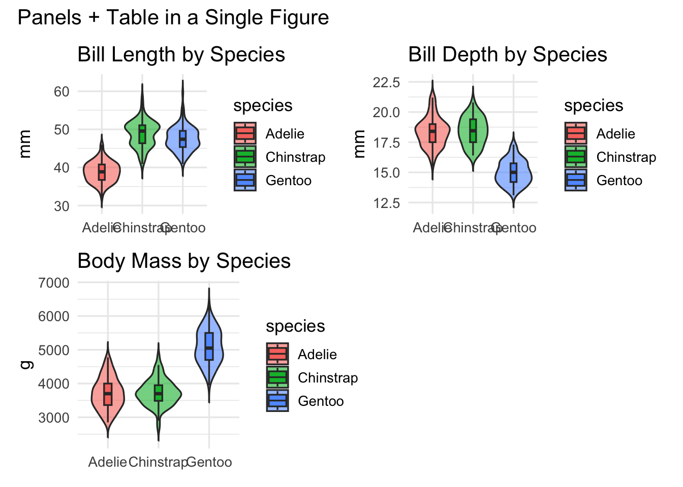
Design guidelines (quick checklist)
- Hierarchy: make the most important panel larger or top-left.
- Consistency: same theme, fonts, and scales where comparisons are intended.
- Economy: collect legends; avoid redundant labels.
- Accessibility: colorblind-safe palettes; sufficient text size.
- Whitespace: breathing room improves readability.
Common pitfalls
- Overcrowding (too many tiny panels).
- Misaligned axes / inconsistent scales.
- Duplicate legends; forgotten units or labels.
- Aspect ratio mismatches creating awkward spacing.
Export: resolution & format
# Vector export (PDF) for print
# ggsave("gc3_multipanel_figure.pdf", plot = pub, width = 11, height = 8.5, device = cairo_pdf)

# High-res PNG for slides
# ggsave("gc3_multipanel_figure.png", plot = pub, width = 11, height = 8.5, dpi = 300)
Tips: Always preview exported figures; ensure labels are legible at final size.
Mini hands-on (optional)
- Take any three plots from your work.
- Compose with patchwork: set widths/heights, collect legends, add a title.
- Aim for one coherent message per figure.
Takeaways
- Layout decisions shape interpretation.
- patchwork provides a clean grammar for multi-plot composition.
- Think in stories: each panel a sentence; the figure the paragraph.
Q&A
Questions, edge cases, or examples from your projects?